Matrizen

Eine Matrix ist eine Anordnung von Einträgen, die als Rechteck dargestellt wird.

Anwendung finden Matrizen unter anderem bei der Lösung von linearen Gleichungssystemen und als Berechnung von linearen Abbildungen.

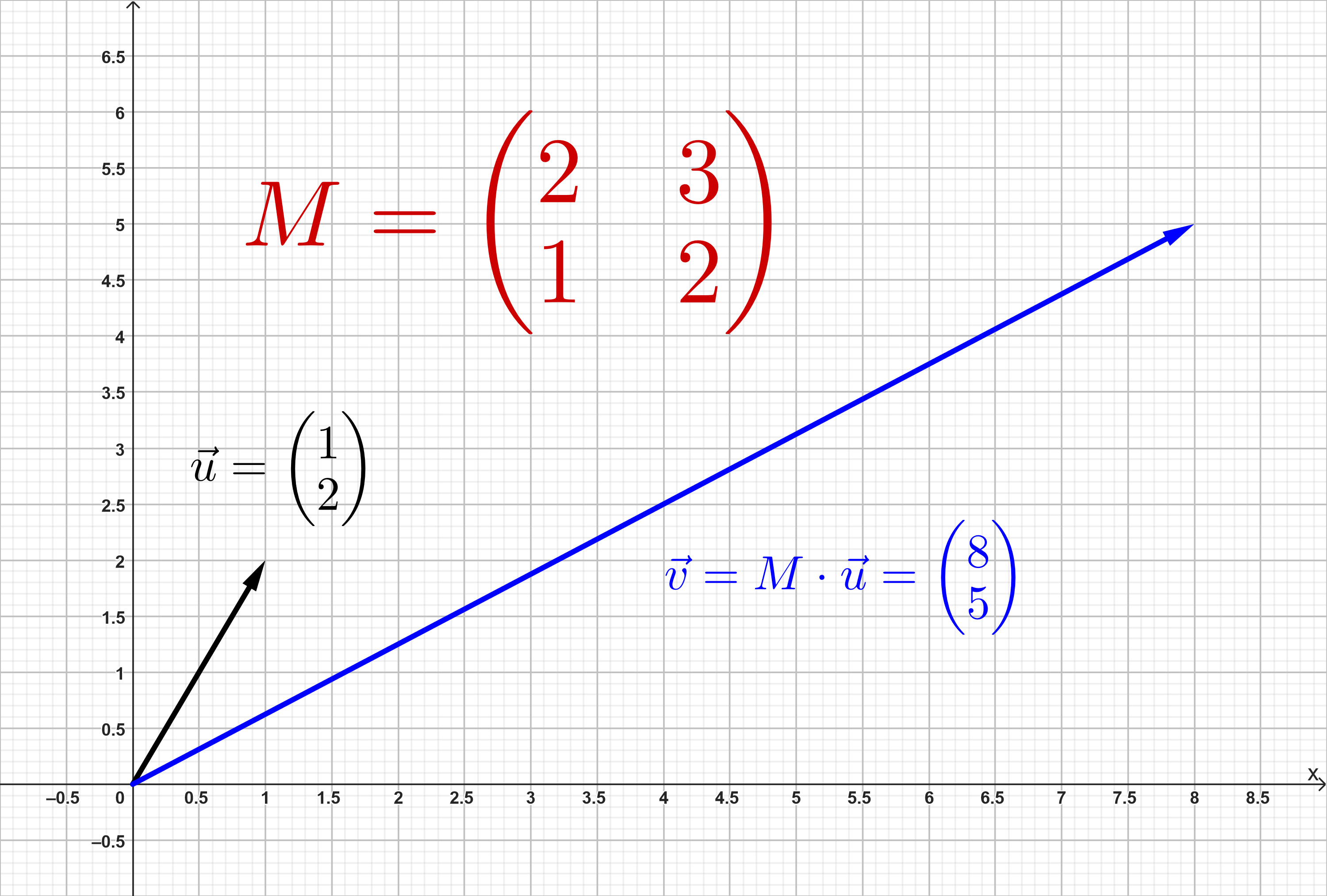
Matrizen beschreiben lineare Abbildungen. Der Vektor $\vec{u}$ wird durch die Matrix $M$ zum Vektor $\vec{v}$ transformiert.

Struktur

A = (\begin{array}{ccc} a_{11} & \dots & a_{1 n} \\ ⋮ & ⋱ & ⋮ \\ a_{m 1} & \dots & a_{m n} \end{array})

$A \in {Mat}_{m \times n}$ ( ${Mat}_{m \times n}$ bezeichnet die Menge aller $m \times n$ Matrizen)

$A$ besteht aus $m$ Zeilen und $n$ Spalten.

Die Einträge $a_{i j}$ nennt man "Elemente".

Ist die Anzahl der Spalten gleich 1, nennt man eine Matrix auch Vektor.

Besondere Matrizen

Nullmatrix

Bei einer Nullmatrix sind alle Elemente Null:

Beispiel: $2 \times 3$ Nullmatrix $\Rightarrow N = (\begin{array}{ccc} 0 & 0 & 0 \\ 0 & 0 & 0 \end{array})$

Einheitsmatrix

Die Einheitsmatrix besitzt in der Diagonale nur Einsen und sonst nur Nullen. Die Größe hängt von der Dimension der Matrix ab.

Beispiel: $3 \times 3$ Einheitsmatrix $\Rightarrow E_{3} = (\begin{array}{ccc} 1 & 0 & 0 \\ 0 & 1 & 0 \\ 0 & 0 & 1 \end{array})$

Diagonalmatrix

Die Diagonalmatrix ist der Einheitsmatrix sehr ähnlich. Sie besitzt nur auf der Diagonale Werte und sonst nur Nullen. Diese Werte müssen aber nicht unbedingt $1$ sein.

$\Rightarrow$ Einheitsmatrix ist eine besondere Diagonalmatrix.

Beispiel: $4 \times 4$ Diagonalmatrix: $(\begin{array}{cccc} 2 & 0 & 0 & 0 \\ 0 & 5 & 0 & 0 \\ 0 & 0 & 8 & 0 \\ 0 & 0 & 0 & 5 \end{array})$

Addition von Matrizen

Es können nur Matrizen mit gleicher Anzahl von Zeilen und Spalten addiert werden.

Die Elemente werden einzeln addiert:

$(\begin{array}{ccc} a_{11} & \dots & a_{1 n} \\ ⋮ & ⋱ & ⋮ \\ a_{m 1} & \dots & a_{m n} \end{array}) + (\begin{array}{ccc} b_{11} & \dots & b_{1 n} \\ ⋮ & ⋱ & ⋮ \\ b_{m 1} & \dots & b_{m n} \end{array}) = (\begin{array}{ccc} a_{11} + b_{11} & \dots & a_{1 n} + b_{1 n} \\ ⋮ & ⋱ & ⋮ \\ a_{m 1} + b_{m 1} & \dots & a_{m n} + b_{m n} \end{array})$

Beispiel für 3x2 Matrizen:

(\begin{array}{cc} 1 & 2 \\ 3 & 4 \\ 5 & 6 \end{array}) + (\begin{array}{cc} 1 & 4 \\ 2 & 5 \\ 3 & 6 \end{array}) = (\begin{array}{cc} 2 & 6 \\ 5 & 9 \\ 8 & 12 \end{array}) = (\begin{array}{cc} 1 + 1 & 2 + 4 \\ 3 + 2 & 4 + 5 \\ 5 + 3 & 6 + 6 \end{array})

Die Matrizenaddition ist assoziativ, kommutativ und besitzt die Nullmatrix als neutrales Element.

Multiplikation mit Skalar

Ein Skalar ist hier eine Zahl. Multipliziert man eine Matrix mit einer Zahl, wird jedes Element mit der Zahl multipliziert:

$s \cdot (\begin{array}{ccc} a_{11} & \dots & a_{1 n} \\ ⋮ & ⋱ & ⋮ \\ a_{m 1} & \dots & a_{m n} \end{array}) = (\begin{array}{ccc} s \cdot a_{11} & \dots & s \cdot a_{1 n} \\ ⋮ & ⋱ & ⋮ \\ s \cdot a_{m 1} & \dots & s \cdot a_{m n} \end{array})$

Beispiel für eine 3x2 Matrix:

3 \cdot (\begin{array}{cc} 1 & 2 \\ 3 & 4 \\ 5 & 6 \end{array}) = (\begin{array}{cc} 1 & 2 \\ 3 & 4 \\ 5 & 6 \end{array}) \cdot 3 = (\begin{array}{cc} 3 & 6 \\ 9 & 12 \\ 15 & 18 \end{array})

Die Multiplikation mit einem Skalar ist kommutativ.

Multiplikation mit einem Vektor

Multipliziert man eine Matrix von links mit einem Vektor, muss die Anzahl der Spalten der Matrix mit der Anzahl der Zeilen des Vektors übereinstimmen.

Um das erste Element des Ergebnisvektors zu erhalten, werden die Elemente der ersten Zeile mit den Elementen des Vektors multipliziert und addiert. Dargestellt an einer 3x3 Matrix und einem 3x1 Vektor:

$A \cdot \vec{v} = (\begin{array}{ccc} a & b & c \\ d & e & f \\ g & h & i \end{array}) \cdot (\begin{array}{c} x \\ y \\ z \end{array}) = (\begin{array}{c} a x + b y + c z \\ d x + e y + f z \\ g x + h y + i z \end{array}) = (\begin{array}{c} b_{1} \\ b_{2} \\ b_{3} \end{array}) = \vec{b}$

$\Rightarrow \begin{array}{c} a x + b y + c z = b_{1} \\ d x + e y + f z = b_{2} \\ g x + h y + i z = b_{3} \end{array}$

Zugehöriges homogenes Gleichungssystem: $A \cdot \vec{v} = 0$

Hilfestellung:

\begin{array}{l} \begin{array}{ccc} x_{1} & \dots & x_{n} \end{array} \\ \begin{array}{cccc} ↓ & ↓ \end{array} \\ (\begin{array}{ccc} a_{11} & \dots & a_{1 n} \\ ⋮ & ⋮ \\ a_{m 1} & \dots & a_{m n} \end{array}) \end{array}

Bei der Multiplikation mit einem Vektor wird immer eine Spalte der Matrix mal dem Vektor genommen.

Stell dir vor, dass der Vektor wie die Zeilen der Matrix waagerecht statt senkrecht liegt und jeweils ein Wert der Matrixzeile und ein Wert des Vektors multipliziert und dann mit einem Plus verbunden werden.

mit $b = (\begin{array}{c} b_{1} \\ ⋮ \\ b_{n} \end{array})$ $\Rightarrow A \cdot \vec{x} = \vec{b}$ $\Rightarrow \sum_{i = 1}^{n} a_{j i} x_{i} = b_{j}$

zugehöriges homogenes System: $\Rightarrow A \cdot \vec{x} = 0 \Rightarrow \sum_{i = 1}^{n} a_{j i} x_{i} = 0$

Multiplikation zweier Matrizen

Um zwei Matrizen multiplizieren zu können, muss die Anzahl der Spalten der linken Matrix gleich der Anzahl der Zeilen der rechten Matrix sein.

Um die Elemente der Ergebnismatrix zu erhalten, multipliziert man die Elemente der jeweiligen Zeile der linken Matrix mit den Elementen der jeweiligen Spalte der rechten Matrix und addiert die Ergebnisse.

Um also das Element $e_{i j}$ zu erhalten, multipliziert man die i-te Zeile der ersten Matrix mit den Elementen der j-ten Spalte der zweiten Matrix und addiert die Ergebnisse.

$(\begin{array}{ccc} a_{11} & \dots & a_{1 n} \\ ⋮ & ⋱ & ⋮ \\ a_{m 1} & \dots & a_{m n} \end{array}) \cdot (\begin{array}{ccc} b_{11} & \dots & b_{1 k} \\ ⋮ & ⋱ & ⋮ \\ b_{n 1} & \dots & b_{n k} \end{array}) = (\begin{array}{ccc} a_{11} \cdot b_{11} + \dots + a_{1 n} \cdot b_{n 1} & \dots & a_{11} \cdot b_{1 k} + \dots + a_{1 n} \cdot b_{n k} \\ ⋮ & ⋱ & ⋮ \\ a_{m 1} \cdot b_{11} + \dots + a_{m n} \cdot b_{n 1} & \dots & a_{11} \cdot b_{1 k} + \dots + a_{m n} \cdot b_{n k} \end{array})$

Beispiel:

$(\begin{array}{ccc} 1 & 2 & 3 \\ 4 & 5 & 6 \end{array}) \cdot (\begin{array}{cc} 1 & 4 \\ 2 & 5 \\ 3 & 6 \end{array}) = (\begin{array}{cc} 1 \cdot 1 + 2 \cdot 2 + 3 \cdot 3 & 1 \cdot 4 + 2 \cdot 5 + 3 \cdot 6 \\ 4 \cdot 1 + 5 \cdot 2 + 6 \cdot 3 & 4 \cdot 4 + 5 \cdot 5 + 6 \cdot 6 \end{array}) = (\begin{array}{cc} 14 & 32 \\ 32 & 77 \end{array})$

Die Multiplikation zweier Matrizen ist nicht kommutativ.

Sie ist aber assoziativ: $(A \cdot B) \cdot C = A \cdot (B \cdot C)$

Sie ist distributiv:

$(A + B) \cdot C = A \cdot C + B \cdot C$

$C \cdot (A + B) = C \cdot A + C \cdot B$

Lineares Gleichungssystem

$\begin{array}{c} a x + b y + c z = b_{1} \\ d x + e y + f z = b_{2} \\ g x + h y + i z = b_{3} \end{array}$

$\Rightarrow A \cdot \vec{v} = (\begin{array}{ccc} a & b & c \\ d & e & f \\ g & h & i \end{array}) \cdot (\begin{array}{c} x \\ y \\ z \end{array}) = \vec{b}$

$\Rightarrow$ Jedes lineare Gleichungssystem lässt sich als Produkt einer Matrix mit einem Vektor schreiben, wobei $A$ die Koeffizientenmatrix darstellt. Um dies zu lösen, wird die erweiterte Koeffizientenmatrix $(A | b) = (\begin{array}{ccc} a & b & c \\ d & e & f \\ g & h & i \end{array} | \begin{array}{c} b_{1} \\ b_{2} \\ b_{3} \end{array})$ benötigt, die man dann entsprechend umformt.

Allgemein

$\begin{array}{c} a_{11} \cdot x_{1} + \dots + a_{n 1} \cdot x_{n} & = b_{1} \\ ⋮ & ⋮ \\ a_{1 m} \cdot x_{1} + \dots + a_{n m} \cdot x_{n} & = b_{m} \end{array}$

$\Rightarrow (\begin{array}{c} a_{11} \cdot x_{1} + \dots + a_{n 1} \cdot x_{n} \\ ⋮ \\ a_{1 m} \cdot x_{m} + \dots + a_{n m} \cdot x_{n} \end{array}) = (\begin{array}{c} b_{1} \\ ⋮ \\ b_{m} \end{array})$

Ein lineares Gleichungssystem lässt sich immer als Produkt einer Matrix mit einem Vektor schreiben.

$A$ nennt man Koeffizientenmatrix vom linearen Gleichungssystem

$\Rightarrow A \cdot \vec{x} = (\begin{array}{ccc} a_{11} & \dots & a_{1 n} \\ ⋮ & ⋱ & ⋮ \\ a_{m 1} & \dots & a_{m n} \end{array}) \cdot (\begin{array}{c} x_{1} \\ ⋮ \\ x_{n} \end{array}) = \vec{b}$

Erweiterte Koeffizientenmatrix

(A | b) = (\begin{array}{ccc} a_{11} & \dots & a_{n 1} \\ ⋮ & ⋮ \\ a_{1 m} & \dots & a_{nm} \end{array} | \begin{array}{c} b_{1} \\ ⋮ \\ b_{n} \end{array})

Um dies zu lösen, benötigen wir die erweiterte Koeffizientenmatrix $(A | b)$ .

Beispiel

$\begin{array}{c} 2 x + 4 y - 5 z = 2 \\ 3 x - 8 z + 4 y = 9 \\ 3 z - 4 x + 4 y = 2 \end{array}$

Bei der Umwandlung in eine erweiterte Koeffizientenmatrix muss man beachten,

dass in der Matrix die Werte vor $x$ , $y$ und $z$ untereinander stehen.

Deshalb ist es von Vorteil, anfangs die Gleichungen zu "sortieren".

\begin{array}{c} 2 x + 4 y - 5 z = 2 \\ 3 x + 4 y - 8 z = 9 \\ - 4 x + 4 y + 3 z = 2 \end{array} \Rightarrow (\begin{array}{ccc} 2 & 4 & - 5 \\ 3 & 4 & - 8 \\ - 4 & 4 & 3 \end{array} | \begin{array}{c} 2 \\ 9 \\ 2 \end{array})

Umformungen

Die Lösung ändert sich nicht bei diesen Umformungen:

Zeilen vertauschen.
Das Vielfache einer Zeile von einer anderen abziehen oder dazu addieren
Zeile durch eine Zahl (ungleich Null) teilen oder mit einem Faktor ungleich $0$ multiplizieren.

Die erweiterte Koeffizientenmatrix kann durch diese Umformungen auf verschiedene Formen gebracht werden. Zu beachten ist, auch die Koeffizienten $b_{1}, \dots, b_{m}$ mit umzuformen. Die häufigste Art, eine solche Matrix zu lösen, ist der Gaußalgorithmus, in dem die Matrix auf Stufenform gebracht wird, sodass sie folgende Form hat:

$(\begin{array}{ccc} 1 & a_{1} & a_{2} \\ 0 & 1 & a_{3} \\ 0 & 0 & 1 \end{array} | \begin{array}{c} b_{1}^{'} \\ b_{2}^{'} \\ b_{3}^{'} \end{array})$

Allgemein

$(\begin{array}{ccccc} a_{11} & \dots & \dots & a_{1 n} & b_{1} \\ 0 & ⋱ & ⋮ & ⋮ \\ ⋮ & ⋱ & ⋮ & ⋮ \\ 0 & \dots & 0 & a_{n n} & b_{n} \end{array})$

Wenn man diese Form erreicht hat, führt man entweder die Matrix wieder auf Gleichungen zurück und löst diese dann oder man formt weiter um. Bei eindeutig lösbaren Gleichungssystemen kann man dann

a_{i j} = {\begin{cases} 1 & f \ddot{u} r i = j \\ 0 & sonst \end{cases}

erreichen, d. h. die Matrix hat in der Diagonale $1$ und sonst überall $0$ .

Rang einer Matrix

Formt man die Matrix zu einer Stufenform um, lässt sich leicht erkennen, welche Zeilen 0 werden. Die Anzahl der Nicht-Nullzeilen ist dann der Rang $r$ der Matrix. Besitzt eine Matrix keine Nullzeile, so hat sie "vollen Rang".

Eine Matrix mit Rang $r$ hat nach den Umformungen also diese Gestalt:

$A = (\begin{array}{cccccc} a_{11} & \dots & \dots & a_{1 r} & \dots & \dots \\ 0 & ⋱ & ⋮ & ⋮ \\ ⋮ & ⋱ & ⋮ & ⋮ \\ 0 & \dots & 0 & a_{r r} & \dots & \dots \\ 0 & \dots & \dots & \dots & \dots & 0 \\ ⋮ & ⋮ \\ 0 & \dots & \dots & \dots & \dots & 0 \end{array})$ Rang von $A = rg (A) = r$

Dabei sind die Diagonalelemente $a_{11}$ bis $a_{r r}$ alle von null verschieden.

Übungsaufgaben

Weitere Aufgaben zum Thema findest du im folgenden Aufgabenordner:
Aufgaben zur Matrix-Vektor-Multiplikation

Dieses Werk steht unter der freien Lizenz
CC BY-SA 4.0 → Was bedeutet das?